Introduction
Traditionally, the input files for the Multi-Objective Reservoir Analyses using Probabilistic Streamflow Forecasts (GRAPS) model are manually created. In addition to this process being meticulous and error-prone, there also was not a way to visualize the network cascade or to easily interact with different parameters associated with the network. This graphical user interface enables GRAPS users to create reservoir networks with intuitive keystrokes and mouse movements. Network files can be saved and opened for editing later, the interface graphics can be exported as a PDF or directly printed, and all input files required to run GRAPS can be exported with the correct information and formatting.
Features of the GRAPS Interface
Reservoir networks are created by placing blocks that correspond to different network nodes (reservoirs, watersheds, junctions, etc.) on the graphics window and then creating links between those blocks. Each network node and link have a unique dialog that stores user-input associated with that node or link. Saving and opening network files and printing network graphics follow a process similar to other desktop applications and exporting input files only requires the user to specify a directory to place the files.
System Requirements
This interface was developed using Python 3.7 and PyQt5. It should be able to run on any Windows, MAC, or Linux operating system as long as the user has a version of Python 3.7 installed as well as PyQt5.
A Note on Units
The user of this interface is responsible for ensuring the units of the values entered correspond with each other (e.g. if storage is provided in acre-feet, inflow should be provided in acre-feet per time step and evaporation depths should be provided in feet). GRAPS makes no assumptions about the units except that they are consistent (i.e. it will not fail if you provide values in mismatched units unless they fall outside the realm of possibility). However, to assist users in setting the model up the dimensions have been provided for each quantity that is to be provided. The dimensions used are M for mass, L for length, and T for time. Combinations of these dimensions will be used to indicate specific types of information to be entered (e.g. L for elevation, L3 for volumes, L3/T for volumetric flowrates, etc…).
Using the GRAPS Interface
Tutorial Video
Interface Layout
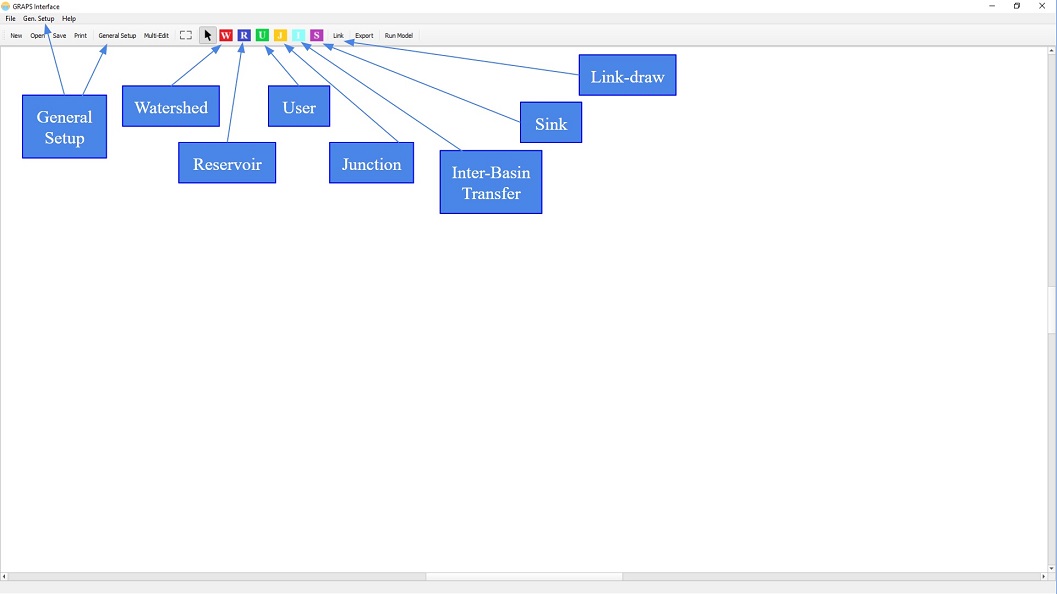
The GRAPS GUI is displayed as a desktop application (Figure 1). A drop-down menu bar is situated at the top of screen and the tool-bar (which the user will interact with the most) directly below it. As indicated in Figure 1, the tool-bar contains buttons for selecting modeling blocks and links as well as generic buttons to create a new file, open an existing file, save the current file, and print the current file. The rectangular button is used to center the screen based on the network that has been drawn and the “Export” button is used to create the input file for GRAPS to run based on the information entered by the user.
General Setup
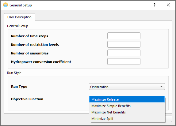
GRAPS requires basic setup information to adequately model the desired scenario. These parameters are entered in the general setup dialog, which is depicted in Figure 2 and Figure 3. This dialog can be accessed either through the “Gen. Setup” menu in the Menu Bar or via the “General Setup” tool bar button. The “General Setup” dialog requires the number of time steps, restriction levels, and ensembles to be entered, as well as the hydropower conversion coefficient.
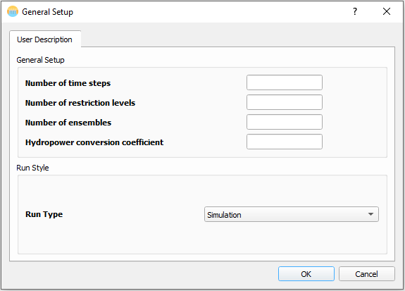
If the run type is selected as simulation, no other information is needed to complete the general setup tab. However, if the run type is set to "Optimization", an objective function must be selected between "Maximum Release", "Maximize Simple Benefits", "Maximize Net Benefits", and "Maximize Spill".
Building Reservoir Networks
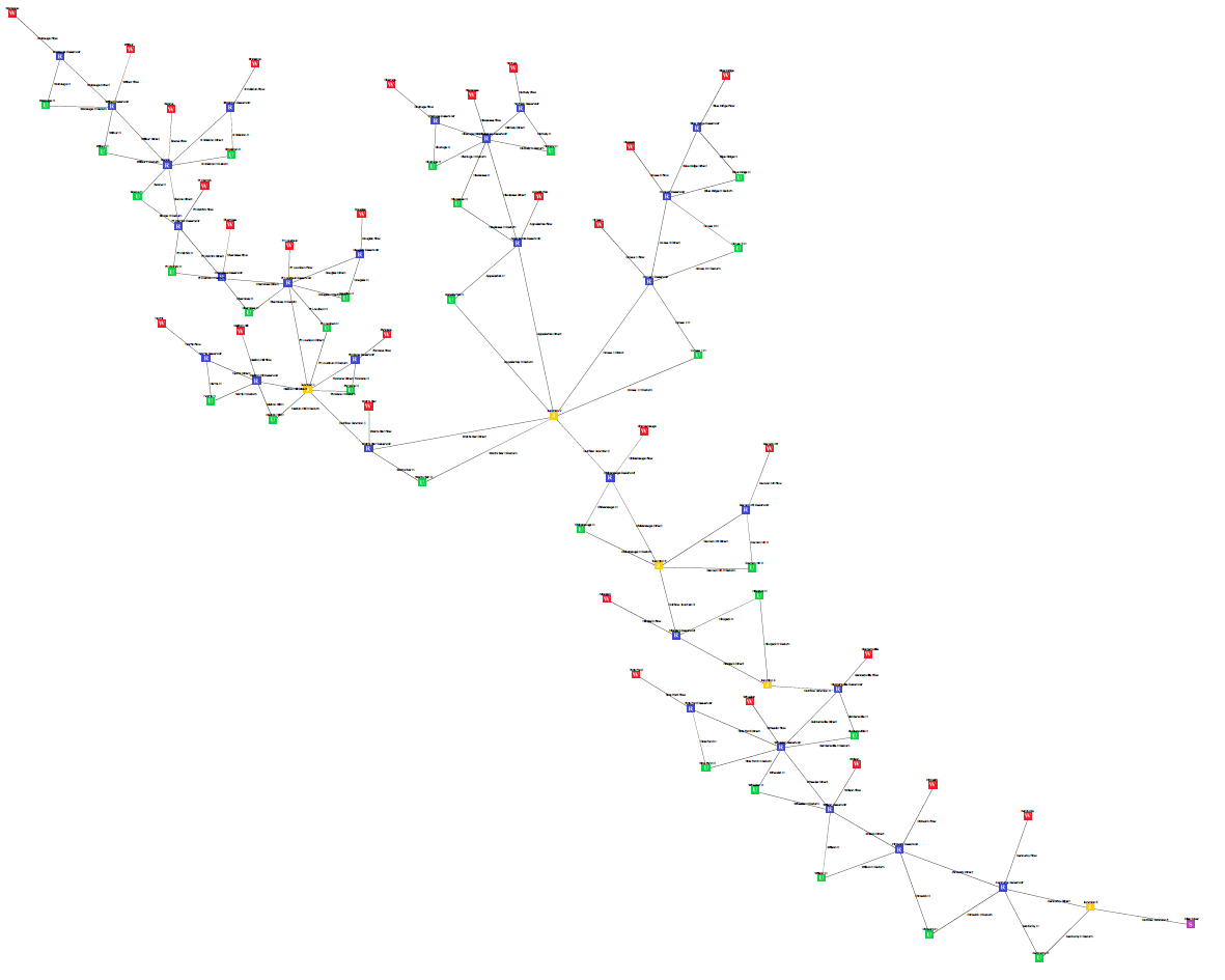
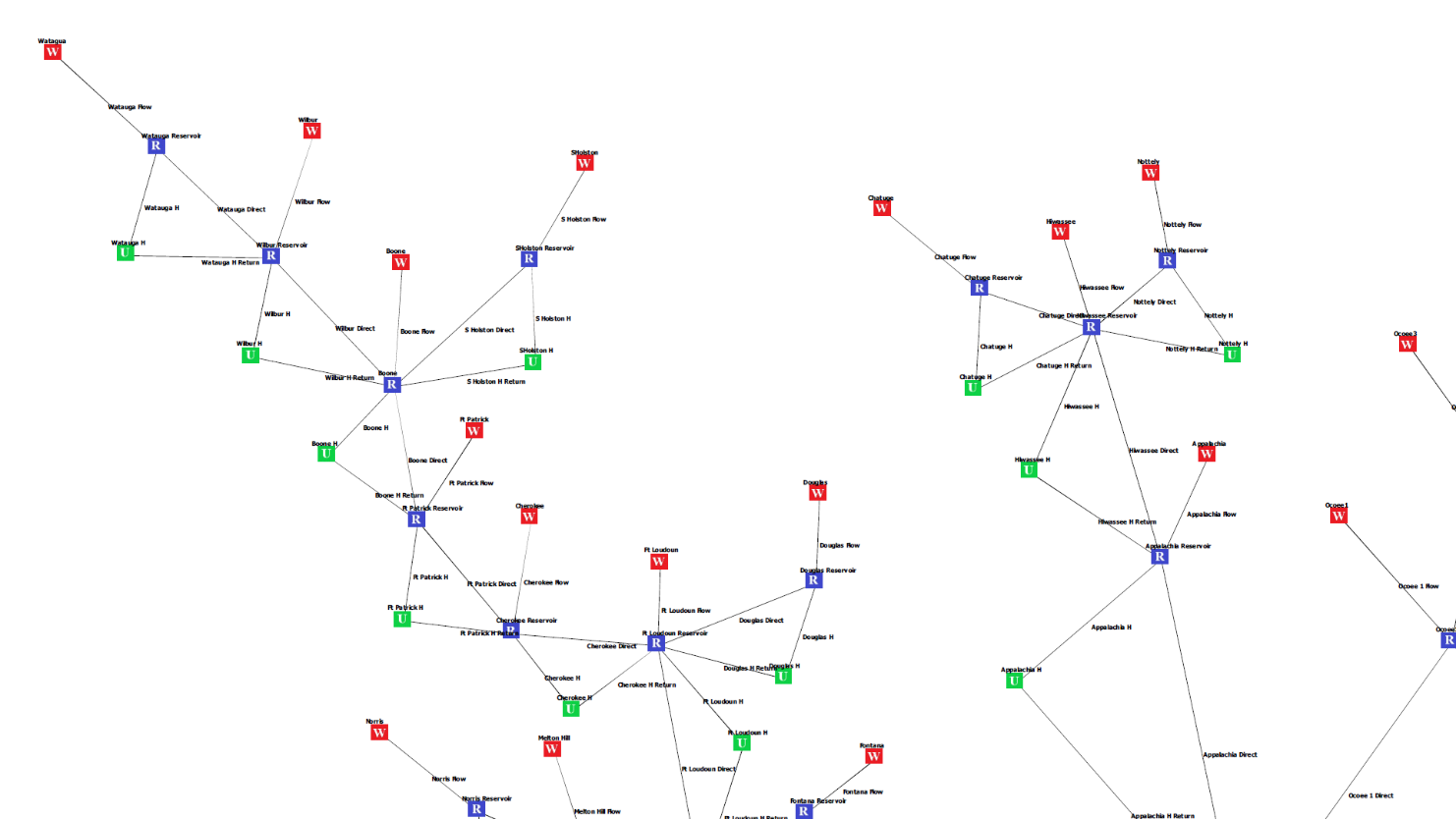
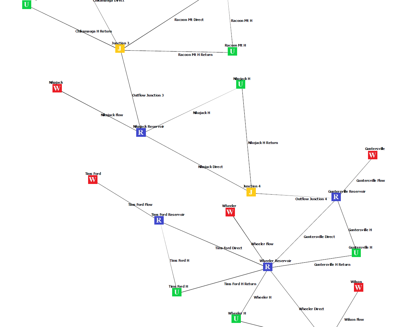
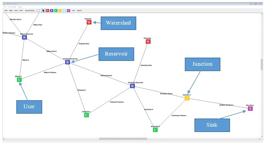
There are six network nodes to be used when creating reservoir networks (Watershed, Reservoir, Inter-basin Transfer, User, Junction, and Sink) as well as Links/Flow connectors. To begin creating networks in GRAPS, first complete the General Setup dialog and then click the toolbar icon corresponding to the name of the first network node you intend to create e.g. the red block with a white “W” for a watershed. To use the mouse without placing nodes, click the mouse pointer tool bar button. An example of some of the downstream main-stem reservoirs in the Tennessee Valley Authority’s (TVA) reservoir network is show in Figure 4 to illustrate a possible network configuration.
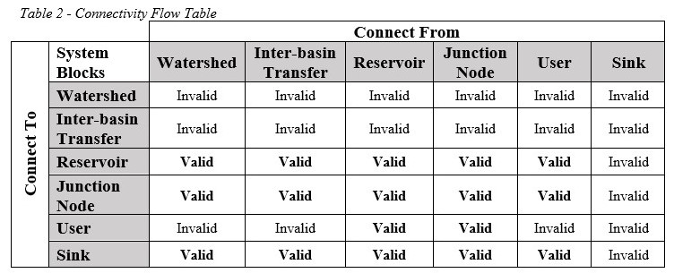
To open the dialog for a node, the node can be double-clicked, or if it is selected with a single click, hitting “Return/Enter” key on the keyboard. Table 2 shows valid and invalid node connection. Though the software should not allow invalid connections, it is best to keep in mind what is valid and what is not.
Watersheds
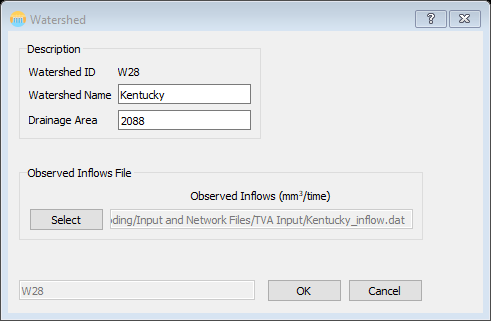
Watersheds provide a description of natural inflows to reservoirs. An example of the watershed dialog is show in Figure 5. The information required in the “Watershed” dialog is the “Watershed Name”, “Drainage Area”, and the user must select a file containing observed inflows. The file must be space delimited (i.e. values separated by white space or tabs) and each line in the file represents one ensemble member and there should be the same number of values as the number of time steps specified in general setup. If you have not specified the number of ensembles to be used, the number is assumed one; therefore, the inflow file should only contain one line of values. For example, if you have specified 5 ensemble members and the number of modeled time steps is 6, your inflow files should look similar to this:
|
10 12 13 15 17 15 12 11 12 16 13 14 13 11 12 13 16 12 11 13 15 15 15 11 10 15 14 17 13 13 |
In the above text box, each line represents an ensemble member and each value in each line represents natural inflow into a watershed for a given time step.
| Table 3 - Watershed Variable Information | ||||
| Variable/Field | Dimension | LB | UB | |
| Drainage Area | L2 | 0.1 | User Defined | |
| Inflows | L3 | 0 | User Defined | |
Variable Information
- Drainage Area - The surface area of which water enters the watershed.
- Inflows - The flow into the watershed per unit of time.
Reservoirs
The information input into the “Reservoir” dialog is essential to effectively running GRAPS. There are four tabs that require user input: “Reservoir Description”, “Evaporation / Storage Relationships”, “Operational Information”, and “Spillway / Outlets”. Each of these tabs is shown below along with a description of what information is required.
Reservoir Description
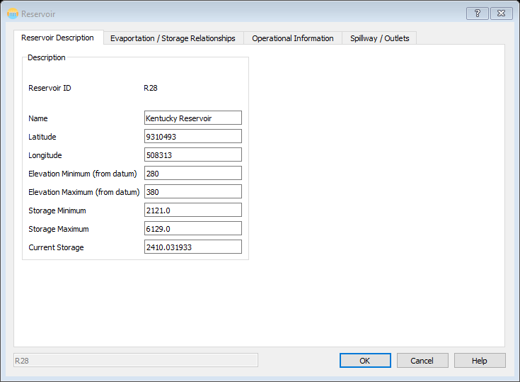
Basic information regarding the reservoir. The most important information for GRAPS are the last 5 fields: min. and max. elevation, min. and max. storage, and current storage.
Reservoir-Evaporation / Storage Relationships
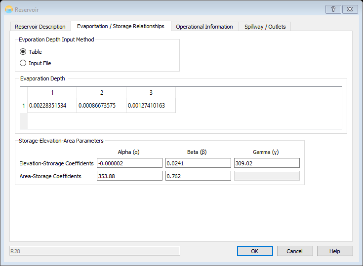
This tab (Figure 7) requires the user input information regarding the lake evaporation depth (in either a table or selecting a file) and the storage relationship coefficients. When simulating over longer periods, it can be easier to use data files rather than manual entry. When “Table” is selected, a table will appear to enter information and when “Input File” is selected, a field to select a file will appear. The below equations (Eqn. 1 - Eqn. 3) explain how the coefficients and the evaporation depths will be used in the model. In the below equations, \({\bar S_{t,t-1}}\) is the average storage between the current and previous time steps, \({\alpha}\), \({\beta}\), and \({\gamma}\) are the coefficients that are requested (they exist separately for each relationship type), and E represents the evaporation depth. All of these quantities are calculated for each reservoir for each time step and ensemble member.
|
Elevation-Storage Relationship |
\[Elev. = \alpha {({\bar S_{t,t - 1}})^2} + \beta ({\bar S_{t,t - 1}}) + \gamma ({\bar S_{t,t - 1}})\] |
Eqn. 1 |
|
Area-Storage Relationship |
\(Area = \alpha {\left( {{{\bar S}_{t,t - 1}}} \right)^\beta }\) |
Eqn. 2 |
|
Evaporation Calculation |
\(Evap. = E \times Area\) |
Eqn. 3 |
Reservoir-Operational Information
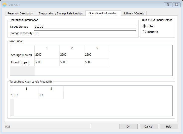
In the “Operational Information” tab (Figure 8) users are required to enter the “Target Storage”, “Storage Probability”, and “Target Restriction Levels Probability” for each restriction level. They are also required to specify a method of entry for the “Rule Curve;” either manual entry of values into a table or selecting a data file. As with the “Evaporation” tab, it is suggested to use the data file input method for long term simulations. Rule curves are not required, but they provide a method for the user to impose realistic, time-varying storage constraints.
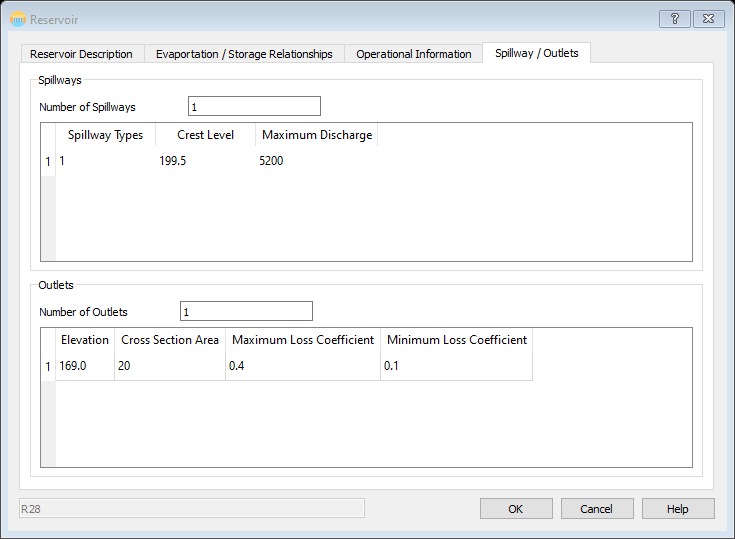
Reservoir-Spillway/Outlets
The “Spillway/Outlets” tab (Figure 9) requires the user enter the “Number of Spillways” and the type, crest level, and maximum discharge for each spillway as well as the “Number of Outlets” and the elevation, cross-sectional area, and maximum and minimum loss coefficients for each outlet. For the “Spillway Type” enter 0 for a controlled spillway or 1 for an uncontrolled spillway.
Variable Information
- Elevation Minimum - The elevation of the lowest point of the reservoir above sea level.
- Elevation Maximum - The elevation of the highest point of the reservoir above sea level.
- Storage Minimum - Used as a lower bound in the calculation for current storage of the reservoir.
- Storage Maximum - Used as an upper bound in the calculation for current storage of the reservoir.
- Current Storage - The initial storage of the reservoir, which is updated each time step of the simulation.
- Evaporation - Represents the water lost from the reservoir due to evaporation for ecah time step.
- Target Storage - The goal storage the reservoir.
- Storage Probability - The probability the reservoir achieves the targes storage.
- Rule Curve - Not required, but adds additional constraints to the probability of meeting the target storage.
- Target Restriction Level Probability - The probability of each restriction level occuring.
- Spillway Type - Either a 0 for a controlled spillway and a 1 for an uncontrolled spillway.
- Crest Level - The elevation above sea level of the crest of the spillway.
- Discharge - Used as an upper bound for a spillway, whereas the spillway discharge cannot exceed this value.
- Elevation - The elevation above sea level of the outlet.
- Cross Sectional Area - The cross sectional area of the outlet.
- Minimum Loss Coefficient - The minimum fraction of water lost from the outlet.
- Maximum Loss Coefficient - The maximum fraction of water lost from the outlet.
Users
The user block is representative of the different types of users that are present in a reservoir network. The user type is selected in the “User” dialog window. If the “User Type” is “Hydropower” the “Hydropower” tab in the “User” description needs to be completed.
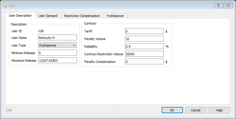
User-User Description
The “User Description” tab (Figure 10) requires the following input: “User Name”, “User Type” (from the drop down box), “Minimum” and “Maximum Release”, “Tariff” amount, “Penalty” amount, “Reliability”, “Contract Restriction Volume”, and the “Penalty Compensation.”
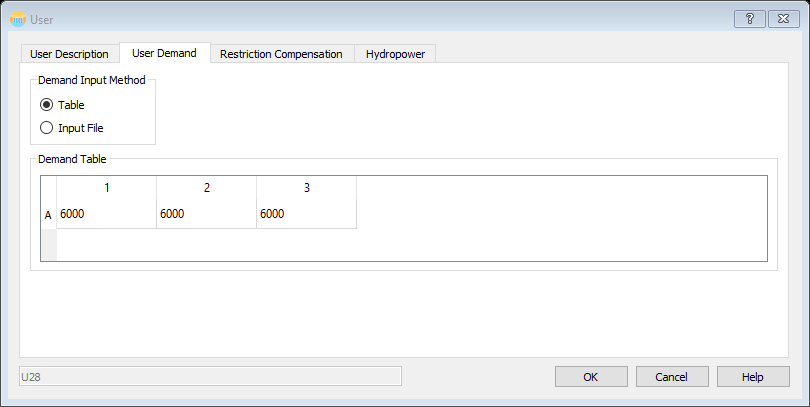
User-User Demand
Again, there is the option to enter the information required in this tab or to select a data file with the information. For larger data sets, it is ideal to use the data file entry method. The information required is the per time step demand for the user. If the model is being run in a simulation mode, these become the releases for that user. If the model is being optimized, these become the starting points for the optimization engine.
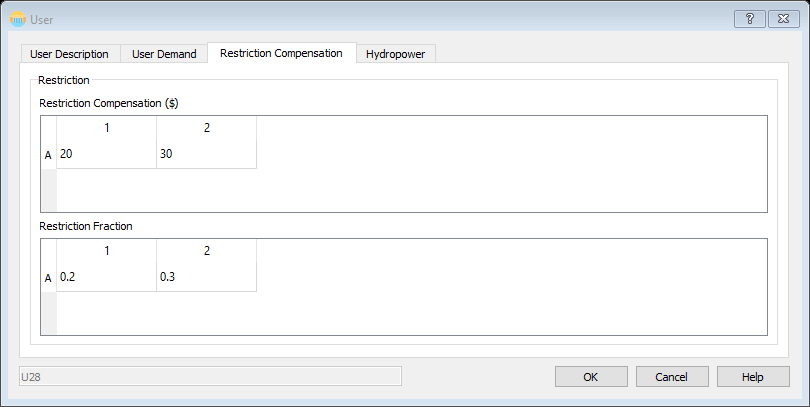
The information required in the “Restriction Compensation” tab is the restriction compensation and fraction for each restriction level.
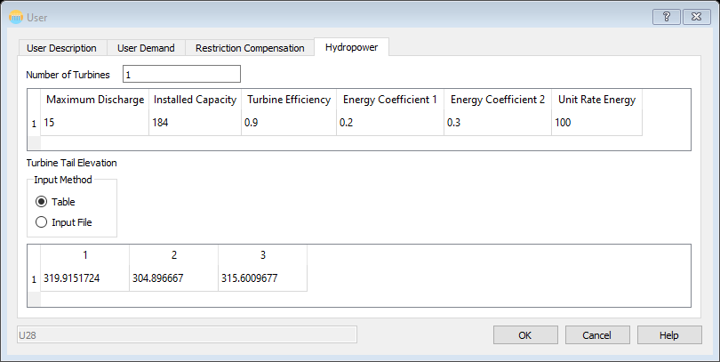
User-Hydropower (Conditional, "User Type")
If the “User Type” is “Hydropower” the “Hydropower” tab becomes required information. The user should specify the “Number of Turbines” and the “Maximum Discharge”, “Installed Capacity”, “Turbine Efficiency”, two energy coefficients, and the “Unit Rate Energy” for each turbine. The “Turbine Tail Elevation” is also required for each time step.
Variable Information
- Minimum Release - An lower constraint on the amount of water the user recieves.
- Maximum Release - An upper constraint on the amount of water the user recieves.
- Tariff - Used to calculate revenue, which is the tariff paid for the release in each time period.
- Penalty Volume - The difference in volume between the contract amount and the threshold for which a penalty is applied.
- Failure Probability (Reliability) - The probability for the user to not meet the penalty volume, which the model uses for optimization.
- Contract Restriction Volume - The volume of water for which the supplier can impose restrictions as part of the contract.
- Penalty Compensation - The tariff given the user fails to recieve the contracted release of water.
- Demand Fraction - The fraction of the demand the particular user uses, which is used to calculate the monthly releases.
- Restriction Compensation - The amount of money given back to the user for each restriction level.
- Restriction Fraction - The fraction of the contracted release of water the user will recieve for each restriction level.
- Maximum Discharge - The maximum volume of water the generator can discharge, which is used as a constraint when calculating net release for the hydropower calculation.
- Installed Capacity - The maximum energy output the generator is rated for.
- Generator Efficiency - The fraction of actual turbine efficiency compared to theoretical, which is kept as a constant for simplicity's sake and used to compute the hydropower.
- Energy Coefficients - Used in the hydropower equation.
- Unit Rate Energy - The price of energy per unit generated.
- Turbine Tail Elevation - The difference between this and the reservoir is taken and used to compute the hydropower.
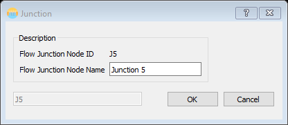
Junctions
Junctions represent a connection between network branches or nodes that have no storage. The only requirement for the “Junction” dialog is the name of the junction.
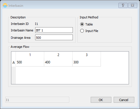
Inter-Basin Transfers
Flows from neighboring basins that could be diverted into the reservoir or a junction. The requirements of the Inter-basin Transfer dialog is the name of the node, the drainage area, and an average flow for each time step. The average flow can either be entered manually in a table or imported with a data file.
| Table 6 - Inter-basin Transfer Variable Information | |||
| Variable/Field | Dimension | LB | UB |
| Drainage Area | L2 | 0.1 | User Defined |
| Average Flow | L3/T | 0 | User Defined |
Variable Information
- Drainage Area - The surface area of which water enters the transfer.
- Average Flow - The average flow through the transfer per time step.
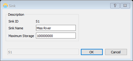
Sinks
Sinks should always be the last node in a network and there should never be more than one. If you desire to have multiple sinks, you can use junction nodes and then tie all the junctions to a single sink. Sinks represent a natural drainage entity such as a large river, sea, or ocean. The required information for the Sink Dialog is the name of the sink and the maximum storage.
| Table 7 - Sink Variable Information | |||
| Variable/Field | Dimension | LB | UB |
| Maximum Storage | L3 | 0.1 | User Defined |
Variable Information
- Maximum Storage - The maximum volume of water a sink may hold.
Links
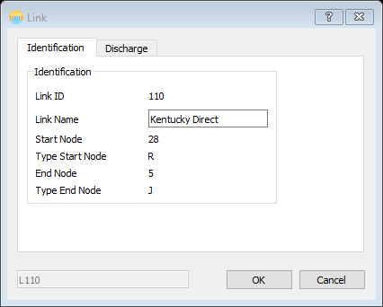
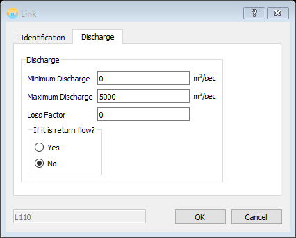
Links are what provides the network connectivity. The “Link” dialog is opened by clicking on the link name and hitting the “Return/Enter” key on the keyboard or double clicking the link name. Each link dialog contains two tabs: “Identification” and “Discharge.” The only requirement on the “Identification” tab is the “Link Name;” the rest of the information will auto-populate. On the “Discharge” tab, the user is required to enter the minimum and maximum discharge, the loss factor, and to specify if it is a return flow or not. If it is a return flow, the number of lags must be specified as well as the values associated with them.
(a)
|
(b)
|
| Figure 17 - Link Dialog (a) Identification tab; (b) Discharge tab | |
Multi-Edit
The Multi-Edit tool allows the user to edit the values of multiple nodes at once. To access it, simply click the Multi-Edit button to the right of the General Setup button on the main toolbar. First, select the type of node which you would like to edit using the drop-down menu at the top right. Then, select the attributes which you would like to edit in the area below. Once selected, it will appear in the main dialog box, and the user can edit a box by simply clicking it and entering the data.
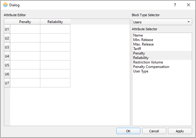
Figure 18 - Multi-Edit Tab
Saving and Reopening Network Files
GRAPS GUI files should always be saved with a `.graps` extension. When you first save a file that will be the default file type. The interface leverages Python’s `pickle` library to serialize the network information. This results in a simple IO mechanism for the interface.
To open a previously saved network, a user can use either the “Open” toolbar icon or the “Open” menu item in the “File” menu in the menu bar. Either option will open a file dialog requiring the user to select what file they wish to open.
The “New” toolbar command will clear the network and all previously set parameters from the current network.
Exporting Input Files and Running a Model
To export the data files needed to run GRAPS, the user must click the “Export” toolbar command. This will prompt the user to select a directory for which to save the files in. There are multiple files that will be created and they will have the names that are required for the model to find them. If you are exporting to a folder with these files already in it, the existing files will be overwritten without warning.
To run a model, simply hit the "Run Model" button on the main toolbar. A dialog then appears, and the user is prompted to navigate to the folder containing the exported files they would like to run, and click "Select Folder". A dialog then confirms that the model has run.
Printing Network Graphics
To print an image of the network open in the interface open the “File” menu in the menu bar and click the “Print” menu item. This will open a traditional print dialog that will allow the user to print the extents of the network to any of the printers available on their machine.
Future Work
While this interface makes new network formulation quicker and simpler, it is not complete. Future additions are integration with the GRAPS model to create a stand-alone modeling package and possible integration with an energy modeling software to allow for more in depth analysis of water management decisions.
References
This document is an adaptation of the “GRAPS Software Documentation” – Dr. Sankar Arumugam. It is meant to be an extension of that document and to provide information regarding the interface and not the GRAPS model.
Example Video
TVA Examples